The Universal Approximation Theorem (UAT) gets quoted constantly, but it is usually described in a fuzzier way than it deserves.
It does not say neural networks are magically good at every task.
It does not say a shallow network is the most practical architecture.
It does not say gradient descent will easily find the right weights.
What it does say is still important:
With a suitable nonlinear activation and enough hidden units, a feedforward network can approximate any continuous function on a bounded domain as closely as we want.
That is a statement about expressive power. In other words, the theorem answers this question:
Can the network represent the function at all, in principle?
That is why the result mattered historically. It killed the idea that neural networks are limited to drawing only simple lines or crude thresholds.
A Common Version of the Theorem
There is not just one single UAT statement. The original result by Cybenko (1989) was written for sigmoidal activations, and later results broadened the allowed activations. A beginner-friendly version is:
Let $K \subset \mathbb{R}^n$ be compact, let $f : K \to \mathbb{R}$ be continuous, and let $\sigma$ be a standard nonlinear activation such as a sigmoid. Then for every $\varepsilon > 0$, there exist an integer $m$ and parameters $a_i \in \mathbb{R}$, $w_i \in \mathbb{R}^n$, $b_i \in \mathbb{R}$, and $c \in \mathbb{R}$ such that
$$ g(x) = \sum_{i=1}^{m} a_i , \sigma(w_i^T x + b_i) + c $$
and
$$ \sup_{x \in K} |f(x) - g(x)| < \varepsilon. $$
That one line is dense, so unpack it:
- Compact means a bounded, closed region such as $[0,1]^n$.
- Continuous means the target function has no jumps inside that region.
- Arbitrarily close means we can make the maximum error as small as we like.
- Existence means the theorem guarantees some parameters exist. It does not tell us how easy they are to find.
- Activation assumptions matter because formal theorem statements put technical conditions on $\sigma$.
- A common modern condition is that $\sigma$ should not be a polynomial, but for intuition it is enough to think of standard nonlinear choices such as sigmoid or ReLU.

Why Nonlinearity Is the Whole Game
Without a nonlinear activation, the theorem fails immediately.
Suppose every hidden unit uses the identity activation $\sigma(z) = z$. In one dimension, even a wide hidden layer collapses to a straight line:
$$ g(x) = \sum_{i=1}^{m} a_i (w_i x + b_i) + c = \left(\sum_{i=1}^{m} a_i w_i\right)x + \left(\sum_{i=1}^{m} a_i b_i + c\right). $$
So width alone does not help. You just get another straight-line rule.
The same collapse happens in higher dimensions. A two-layer network becomes
$$ g(x) = W_2(W_1 x + b_1) + b_2 = (W_2 W_1)x + (W_2 b_1 + b_2). $$
That is still just an affine map. In plain English, it is one overall linear transformation plus a shift.
So even if you make the hidden layer extremely wide, a network with only identity activations cannot bend into a complicated curve. It collapses into one overall affine transformation.
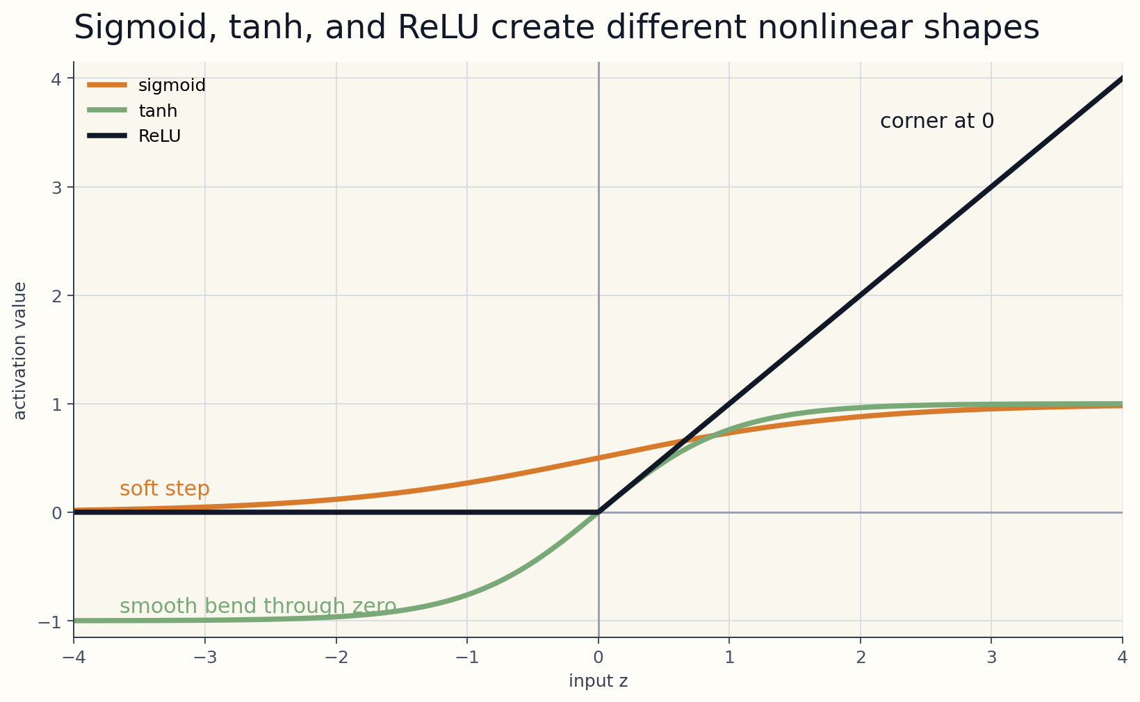
This is the reason activations such as sigmoid, tanh, and ReLU matter so much. They let the network create bends, steps, corners, and local regions. Width then gives you more of those building blocks.
Intuition: Hidden Units Build Small Local Features
The proof ideas behind UAT are mathematical, but the intuition is simpler than the formal statement.
All the pictures below are one-dimensional because they are easier to draw. The actual theorem still applies to functions of many variables.
Think of each hidden unit as producing a small shape:
- a soft step
- a hinge
- a local bump
- a region that turns on and off
For example, with a sigmoid $\sigma(z)$, one soft step is
$$ s(x; t, k) = \sigma(k(x - t)). $$
If $k$ is large, that step becomes sharp near the threshold $t$.
Now subtract two such steps:
$$ b(x; u, v, k) = \sigma(k(x-u)) - \sigma(k(x-v)). $$
That gives a soft bump which is near zero outside the interval $[u,v]$ and higher inside it.
Once you have several such bumps, the output layer can add them:
$$ g(x) = \sum_{j=1}^{m} c_j , b(x; u_j, v_j, k_j). $$
This is not the full theorem, but it is the right mental model. Hidden units create reusable local pieces, and the final layer combines them into a more complicated shape.

Here is the same idea plotted directly from the equations with Python and Matplotlib:
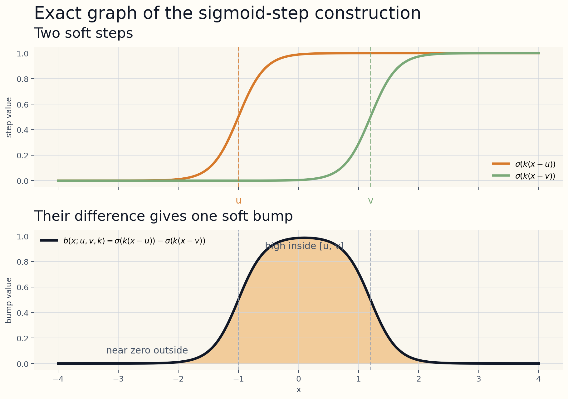
u and one at v. Bottom: their difference, which creates a single soft bump that is high inside [u, v] and near zero outside.Here $u$ and $v$ decide where the bump turns on and off, while $k$ controls how sharp the two edges are.
import numpy as np
import matplotlib.pyplot as plt


def sigma(z):
    return 1.0 / (1.0 + np.exp(-z))


def soft_step(x, t, k):
    return sigma(k * (x - t))


def bump(x, u, v, k):
    return soft_step(x, u, k) - soft_step(x, v, k)


u = -1.0
v = 1.2
k = 4.5
x = np.linspace(-4, 4, 1200)

s_u = soft_step(x, u, k)
s_v = soft_step(x, v, k)
b = bump(x, u, v, k)

fig, axes = plt.subplots(2, 1, figsize=(10, 7), sharex=True, constrained_layout=True)

axes[0].plot(x, s_u, label=r"$\sigma(k(x-u))$")
axes[0].plot(x, s_v, label=r"$\sigma(k(x-v))$")
axes[0].axvline(u, linestyle="--")
axes[0].axvline(v, linestyle="--")
axes[0].set_title("Two soft steps")
axes[0].legend()

axes[1].plot(x, b, color="black", label=r"$b(x;u,v,k)$")
axes[1].fill_between(x, 0, b, alpha=0.3)
axes[1].axvline(u, linestyle="--")
axes[1].axvline(v, linestyle="--")
axes[1].set_title("Their difference gives one soft bump")
axes[1].legend()

plt.show()
The ReLU Version: Piecewise Linear Approximation
Modern networks often use ReLU instead of sigmoid:
$$ \operatorname{ReLU}(x) = \max(0, x). $$
In one dimension, sums of shifted ReLUs generate piecewise linear functions:
$$ g(x) = \alpha_0 + \alpha_1 x + \sum_{j=1}^{m} \beta_j , \operatorname{ReLU}(x - t_j). $$
This is still a one-hidden-layer ReLU network. It is just written in a form that makes the piecewise-linear structure easier to see.
Each extra term introduces another place where the slope can change. So as you add more hidden units, the network can place more breakpoints and better follow a curved target.
That is why ReLU networks are still universal approximators even though they do not look like the older sigmoid proofs.
Worked Example on $[0,1]$
Take this target function:
$$ f(x) = 0.50 + 0.22 \sin(2\pi x - 0.35) + 0.08 \sin(6\pi x + 0.30), \qquad x \in [0,1]. $$
It is smooth, continuous, and definitely not just a straight line.
To build intuition, imagine approximating it with piecewise linear fits, which is exactly the kind of shape a 1D ReLU network is good at producing.
- A purely linear model can only draw one segment.
- A small network can place a few bends and catch the rough trend.
- A wider network can place many bends and push the error down across the whole interval.
In the illustration below, the same target curve is approximated at three different capacities. The maximum error drops from about 0.322 to 0.182 to 0.013 as we allow more bends. Because the target curve itself only moves within a fairly small vertical range, 0.322 is visibly poor while 0.013 is already quite close.

What the Theorem Does Not Promise
This part is where people often overread the result.
The UAT does not guarantee:
- that one hidden layer is the most parameter-efficient architecture
- that the network will learn the approximation from finite data
- that gradient descent will find the right parameters quickly
- that the required width will be small
- that every possible function is covered by the classic statement
The standard theorem is about approximating continuous functions on compact domains. That is already a big result, but it is not the same thing as saying “neural networks can do anything with no tradeoffs.”
Why Deep Networks Still Matter If a Shallow One Is Universal
This is the next natural question.
If one hidden layer is universal, why do people build deep networks at all?
Because universality is not efficiency.
A shallow network may need an absurd number of hidden units to represent a function compactly. A deeper network can often reuse intermediate structure and reach the same approximation with far fewer parameters.
That is especially important for:
- hierarchical patterns in images
- compositional structure in language
- reusable features in speech and time series
- algorithm-like computations with many stages
So the UAT says shallow networks are expressive enough in principle, while modern deep learning is mostly about doing the job efficiently and trainably.
Final Takeaway
The Universal Approximation Theorem is best understood as a representational guarantee:
A neural network with a suitable nonlinear activation and enough width can approximate any continuous function on a bounded region to arbitrary accuracy.
That is why neural networks are fundamentally more flexible than linear models.
The theorem does not solve optimization, data efficiency, or generalization. But it does establish something essential:
Neural networks are not limited by a lack of expressive power.
Once that door is open, the real engineering questions become how to learn the approximation well, how much capacity to use, and which architecture gets there with the least pain.