Large Language Models (LLMs) such as GPT-2, GPT-3, LLaMA, and BERT are built on top of the Transformer architecture. That architecture changed natural language processing by replacing recurrence with attention, which lets models process sequences more efficiently and capture long-range relationships more directly.
If you are trying to understand what terms like layer, transformer block, and attention head actually mean, the easiest way is to follow the path a sentence takes through a GPT-style model.
One terminology note before we begin: in most GPT-style model specifications, a layer usually means one full transformer block. So if a model is described as having 48 layers, that usually means it has 48 stacked transformer blocks.
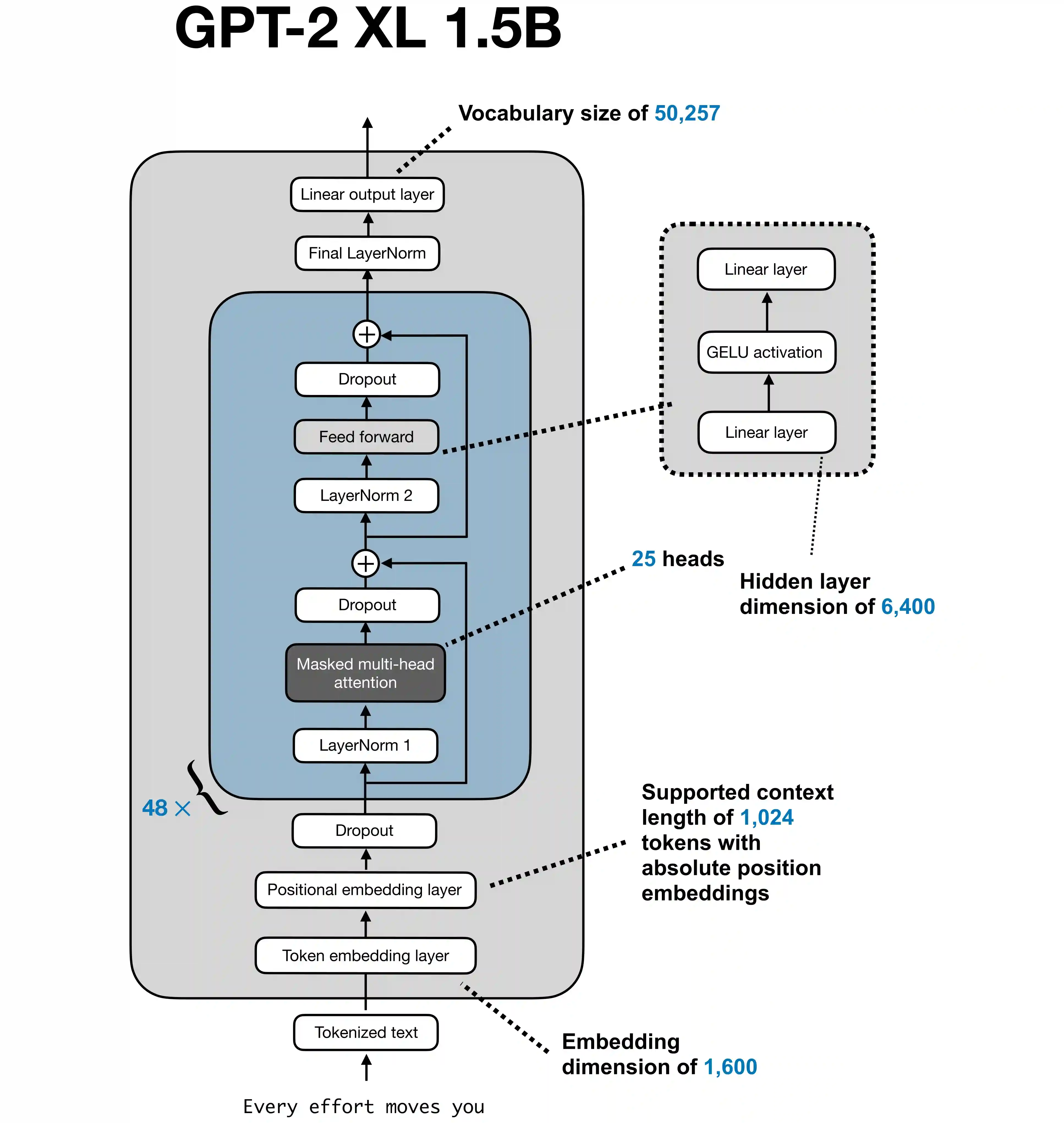
GPT-2 XL as a concrete example: 48 transformer blocks, 25 attention heads, 1,600-dimensional token embeddings, a 6,400-dimensional MLP expansion, and a 1,024-token context window.
The High-Level Pipeline
At a high level, a transformer language model processes text like this:
Input text
  -> Tokenization
  -> Token embeddings + positional information
  -> N stacked transformer blocks
  -> Final hidden state
  -> Linear projection to vocabulary
  -> Softmax
  -> Next-token probabilities
The core idea is simple: each block refines the representation of every token, and the final layer turns those representations into a probability distribution over the vocabulary.
1. Tokenization: Turning Text Into Model Inputs
Before text enters the model, it is broken into tokens.
For example, the sentence:
The cat sat on the mat
might be represented as whole-word-like tokens, or as smaller subword pieces depending on the tokenizer. Each token is then mapped to a numeric token ID.
This matters because the model never sees raw text directly. It only sees a sequence of token IDs.
2. Embedding Layer
Each token ID is converted into a dense vector called an embedding.
If a model has a hidden size of d_model = 1600, then every token becomes a 1,600-dimensional vector.
For GPT-2 XL, that 1,600-dimensional vector is the model’s base representation size. The rest of the network keeps transforming vectors of this size as the text moves upward through the stack.
These embeddings are learned during training, which is why tokens with related meanings often end up with related vector patterns.
3. Positional Information
Transformers process tokens in parallel, so they need some way to represent order.
That is why the model adds positional information to token embeddings.
Conceptually:
input_representation = token_embedding + positional_information
Older GPT-style models such as GPT-2 use learned absolute positional embeddings. Many newer LLMs use alternatives such as RoPE instead. The purpose is the same: the model must know the difference between:
dog bites manman bites dog
without relying on recurrence.
4. Transformer Blocks: The Core of the Model
After embeddings are prepared, they pass through many stacked transformer blocks:
Embeddings
  -> Block 1
  -> Block 2
  -> Block 3
  -> ...
  -> Block N
Each block takes the previous representation and produces a more contextual one.
Typical model depths look like this:
| Model | Approximate Layers |
|---|---|
| GPT-2 XL | 48 |
| GPT-3 | 96 |
| LLaMA-2 | 32 to 80 |
The deeper the stack, the more opportunities the model has to refine syntax, relationships, and abstract meaning.
5. What Is Inside a Transformer Block?
A GPT-style transformer block typically contains:
- Layer normalization
- Masked multi-head self-attention
- A residual connection
- Another layer normalization
- A feed-forward network, often called an MLP
- Another residual connection
A simplified flow looks like this:
Input
  -> LayerNorm
  -> Multi-Head Self-Attention
  -> Residual Add
  -> LayerNorm
  -> Feed-Forward Network
  -> Residual Add
  -> Output
This pattern repeats for every block in the model.
6. Self-Attention: How Tokens Look at Other Tokens
Self-attention is the mechanism that lets each token decide which other tokens matter.
Consider the sentence:
The animal didn't cross the street because it was tired.
To interpret it, the model needs to connect it to animal. Attention gives the model a way to learn that relationship.
Each token is projected into three vectors:
- Query (Q): what this token is looking for
- Key (K): what this token can offer
- Value (V): the information this token contributes
The standard attention formula is:
Attention(Q, K, V) = softmax((QK^T) / sqrt(d_k))V
In plain English:
- compare each query with all keys
- turn those scores into weights
- use the weights to mix the value vectors
That produces a contextual representation for each token.
7. Multi-Head Attention
Instead of computing attention once, transformers compute it multiple times in parallel using attention heads.
Each head gets a different learned projection of the same input, so different heads can specialize in different patterns.
Possible behaviors include:
| Head | Possible Focus |
|---|---|
| Head 1 | local syntax |
| Head 2 | subject-verb agreement |
| Head 3 | pronoun resolution |
| Head 4 | long-range dependencies |
These roles are not fixed by design, but they are a useful intuition for why multiple heads help.
8. Why Hidden Size and Head Count Must Match
The model’s hidden dimension is split across attention heads:
hidden_size = number_of_heads x head_dimension
For GPT-2 XL:
hidden_size = 1600number_of_heads = 25head_dimension = 1600 / 25 = 64
So each head works on a 64-dimensional slice, and the outputs of all 25 heads are concatenated back together into the original 1,600-dimensional space.
This is why head count is not arbitrary. It must divide cleanly into the model’s hidden size.
9. The Feed-Forward Network (MLP)
After attention, each token passes through a feed-forward network. This is often the second major component inside each transformer block.
The usual structure is:
Linear
  -> Activation
  -> Linear
For GPT-2 XL, the MLP expands the 1,600-dimensional representation to a larger internal size and then projects it back down:
1600 -> 6400 -> 1600
In many modern models, the activation function is GELU or SwiGLU.
Unlike attention, which mixes information across tokens, the MLP operates independently on each token position. Its job is to add nonlinear transformation capacity after attention has gathered context.
10. Residual Connections and Layer Normalization
Residual connections are critical in deep transformers.
The idea is:
output = sublayer(x) + x
This helps because it:
- stabilizes optimization
- improves gradient flow
- makes very deep networks trainable
Layer normalization helps keep activations well-behaved as they move through dozens of stacked blocks.
Without residual connections and normalization, modern LLMs would be much harder to train reliably.
11. The Output Layer
After the final transformer block, the model produces a hidden state for each token position. To predict the next token, it takes the final hidden state for the current position and projects it into vocabulary space.
The flow is:
Final hidden state
  -> Linear projection
  -> Softmax
  -> Probability distribution over the vocabulary
For GPT-2 XL, that vocabulary size is 50,257 tokens.
The token with the highest probability may be selected, or decoding strategies such as sampling, top-k, or nucleus sampling may be used instead.
12. Autoregressive Generation
GPT-style models are autoregressive. They generate one token at a time.
If the prompt is:
The capital of France is
the model predicts the next token, such as:
Paris
Then that new token is appended to the sequence, and the model predicts again.
So generation works like this:
Token 1 -> Token 2 -> Token 3 -> ...
This is why inference is sequential across generated tokens, even though much of the computation inside each step is highly parallel.
13. What Runs Sequentially and What Runs in Parallel?
This distinction is one of the most important ideas in transformer systems.
Sequential Parts
Some parts cannot be parallelized across depth or generation steps:
- Stacked transformer blocks
Block 2 needs the output of Block 1, so the blocks run one after another.
- Autoregressive decoding
When generating text, the model must produce the next token before it can produce the one after that.
Parallel Parts
A lot still happens in parallel inside each step:
- Attention heads
All heads in a multi-head attention module run in parallel.
- Token computations during training and prefill
Tokens in the input sequence are processed in parallel inside a block.
- MLP computation across tokens
The feed-forward network is applied independently to each token position, which makes it highly parallelizable.
A simplified picture looks like this:
Tokens in a sequence (parallel)
  -> Transformer Block 1
     -> Attention heads (parallel)
     -> Token positions (parallel)
     -> MLP on each token (parallel)
  -> Transformer Block 2
  -> ...
  -> Output probabilities
This combination of sequential depth and massive internal parallelism is a big reason transformers scale so well on GPUs.
14. Why Stacking Many Layers Works
Different layers often capture different kinds of information.
A common intuition is:
| Layer Region | Tends to Emphasize |
|---|---|
| Early layers | local patterns, token identity, short-range syntax |
| Middle layers | phrase structure, dependencies, compositional relationships |
| Later layers | higher-level semantics, task signals, prediction-ready features |
This is not a hard rule, but it is a useful mental model. Each block refines what the model knows about every token by mixing context and applying nonlinear transformations again and again.
15. A Quick Note on BERT vs GPT-Style Models
BERT and GPT both use transformer blocks, but they differ in how attention is applied:
- BERT uses bidirectional attention, so tokens can attend to both left and right context.
- GPT-style models use causal masking, so tokens can attend only to earlier positions when predicting the next token.
That difference is one reason BERT is mainly used for understanding tasks, while GPT-style models are naturally suited for generation.
Final Takeaway
The internal structure of an LLM is complex, but the main idea is elegant:
- text becomes token IDs
- token IDs become embeddings
- embeddings pass through many transformer blocks
- each block applies attention and an MLP
- the final representation is projected into vocabulary probabilities
Once you understand layers, transformer blocks, attention heads, hidden dimensions, and execution parallelism, the architecture of modern LLMs becomes much easier to reason about.
That foundation also makes it easier to study more advanced topics such as scaling laws, KV cache design, inference optimization, long-context attention, and model interpretability.