The KV cache is one of those LLM inference terms that sounds simple until someone asks you to explain it from first principles.
At a high level, the idea is:
During generation, a transformer stores the previously computed key and value vectors, so it does not recompute them for the whole sequence every time it predicts the next token.
That is the short answer. But the short answer hides the important part: why keys and values are reusable, why queries are not cached in the same way, and why this matters so much for latency.
In this post, I explain KV cache from the attention matrix level. If you want the broader background first, read my earlier posts on Q, K, and V vectors in attention, attention mechanisms, and LLM inference basics: prefill, decode, TTFT, and ITL.
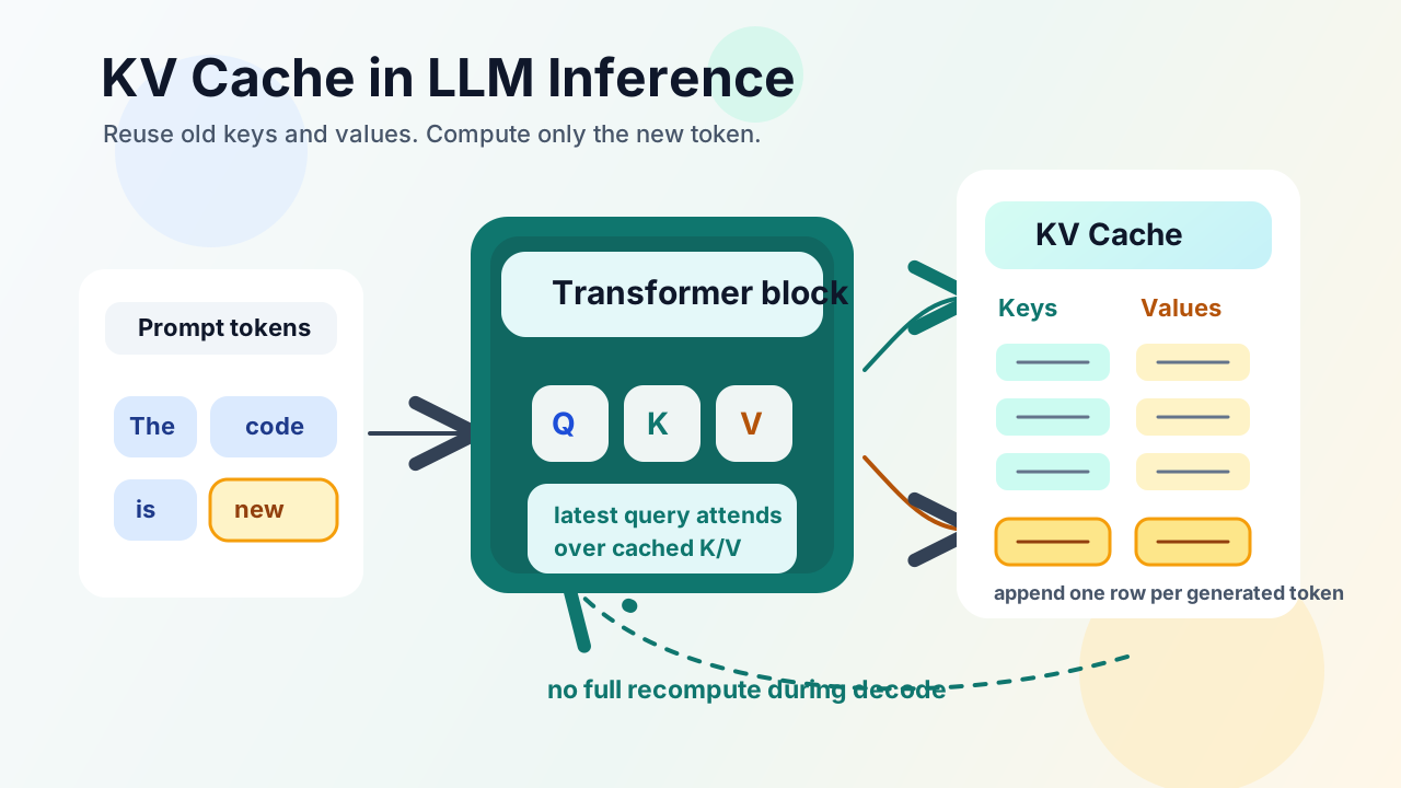
During decode, the model does not rebuild the whole attention state from scratch. It computes the new token’s query, key, and value, appends the new key and value to the cache, and attends over the cached history.
Where KV Cache Appears
KV cache is an inference-time optimization.
It is not the main story during pretraining. During pretraining, the model is learning its weights. During inference, the weights are already fixed and the model is generating tokens from a prompt.
For a decoder-only LLM, generation has two important phases:
- Prefill: process the full input prompt and produce the first output token.
- Decode: generate the remaining output tokens one at a time.
The KV cache is created during prefill and then reused during decode.
This matters because user-facing latency is shaped by the same split:
- long prefill usually increases time to first token
- slow decode usually increases inter-token latency
I covered those metrics separately in TTFT in LLMs Explained. KV cache is one of the reasons decode can be fast enough to stream text interactively.
The Tiny Example
Assume the prompt is:
The code is
For simplicity, treat this as three tokens:
["The", "code", "is"]
Also assume each token embedding has 4 dimensions. Then the input matrix X has shape:
X = 3 x 4
In a transformer attention layer, the input is projected into three matrices:
Q = X WQ
K = X WK
V = X WV
If WQ, WK, and WV are each 4 x 4, then:
Q = 3 x 4
K = 3 x 4
V = 3 x 4
These are the query, key, and value matrices. I already explained the intuition in the Q/K/V article, but the short version is:
Qasks what each token is looking forKdescribes what each token can match againstVcarries the information that will be mixed into the output
What Happens During Prefill
In prefill, the model processes all prompt tokens together.
The attention scores are computed as:
scores = Q K^T
With our toy shapes:
Q      = 3 x 4
K^T    = 4 x 3
scores = 3 x 3
After scaling, masking, and softmax, we get attention weights:
weights = 3 x 3
Then the model mixes the values:
context = weights V
With shapes:
weights = 3 x 3
V       = 3 x 4
context = 3 x 4
Every row in the context matrix corresponds to a token position. To predict the next token after:
The code is
the model only needs the last row of this context matrix, because the next-token prediction is made from the final position.
That final context vector is projected to logits over the vocabulary, and from those logits the model picks the next token. Suppose the next token is:
running
Now the running sequence is:
The code is running
This is where the decode phase begins.
The Naive Decode Path
Without thinking about KV cache, we might recompute everything from scratch for the longer sequence.
Now there are four tokens, so:
X = 4 x 4
Then:
Q = 4 x 4
K = 4 x 4
V = 4 x 4
The attention scores would be:
Q K^T = (4 x 4)(4 x 4) = 4 x 4
Then:
weights = 4 x 4
context = (4 x 4)(4 x 4) = 4 x 4
Finally, we again use only the last row of the context matrix to predict the next token.
This works, but it wastes work.
The first three tokens did not change:
The
code
is
Their key and value vectors were already computed during prefill. Recomputing them during every decode step is redundant.
The First Key Insight: Only the Last Context Vector Is Needed
During decode, the model is trying to predict the next token from the latest position.
So it does not need the full new context matrix. It only needs:
context vector for the latest token
If the latest token is:
running
then the model only needs the context vector for running.
To get that one context vector, the model needs:
- the attention weights for the latest token
- the value vectors for all tokens so far
In shape terms:
latest attention weights = 1 x 4
full V matrix            = 4 x 4
latest context vector    = 1 x 4
So we do not need all rows of attention weights. We only need the row for the newest token.
The Second Key Insight: Past Keys and Values Do Not Change
How do we get the attention weights for the latest token?
We compare the latest token’s query with all keys:
latest scores = q_latest K_full^T
In shape terms:
q_latest = 1 x 4
K_full^T = 4 x 4
scores   = 1 x 4
This tells us something important:
- we need only the latest query
- we need the full key matrix
- we need the full value matrix
But the full key and value matrices contain old rows plus one new row.
For:
The code is running
the keys and values for The, code, and is were already computed during prefill. Only the key and value for running are new.
So the efficient decode path is:
- Take only the newest token embedding.
- Compute its
q,k, andv. - Append the new
kto the cached keys. - Append the new
vto the cached values. - Use the latest
qagainst the full cachedK. - Use the resulting attention weights against the full cached
V. - Produce the latest context vector and predict the next token.
That stored collection of previous keys and values is the KV cache.
Why It Is Called KV Cache, Not QKV Cache
This is a common interview question.
The model caches keys and values because it needs all past keys and values at every decode step.
It does not usually cache queries for the same purpose because, at the next decode step, the model only needs the query for the newest token.
The older queries helped produce older context vectors. But those older context vectors are not needed again for the next-token prediction. The next prediction is based on the newest position only.
So the reusable state is:
past K
past V
not:
past Q
That is why the optimization is called key-value cache.
Prefill With KV Cache
During prefill, the model processes the whole prompt:
The code is
It computes:
K_prompt
V_prompt
and stores them.
So after prefill, the cache contains:
K cache = keys for [The, code, is]
V cache = values for [The, code, is]
The model then predicts the first output token, for example:
running
Decode With KV Cache
During the next decode step, the model does not reprocess the entire sequence from scratch.
It takes only:
running
and computes:
q_running
k_running
v_running
Then it appends:
K cache = keys for [The, code, is, running]
V cache = values for [The, code, is, running]
Now the latest query attends over the full key cache:
q_running -> K cache
and the resulting attention weights mix the full value cache:
attention weights -> V cache
The output is the context vector for running, which is used to predict the next token, maybe:
fast
Then the process repeats.
What KV Cache Saves
KV cache saves redundant computation.
Without it, every decode step would repeatedly compute keys and values for the full growing sequence:
step 1: prompt tokens
step 2: prompt tokens + token 1
step 3: prompt tokens + token 1 + token 2
step 4: prompt tokens + token 1 + token 2 + token 3
With KV cache, each decode step only computes keys and values for the newest token and reuses the past.
This is a big reason autoregressive generation is practical. The model still has to attend over the growing history, but it avoids repeating the projection work for old tokens again and again.
For a chatbot, this directly affects how fast the answer streams. Lower decode cost usually means better inter-token latency.
The Tradeoff: KV Cache Uses Memory
The KV cache is not free.
It stores keys and values for:
- every token in the prompt
- every generated token so far
- every transformer layer
- attention heads, depending on the attention variant
- every active request in the batch
So the cache can become large. Long-context models especially put pressure on GPU memory and memory bandwidth.
This is why attention variants such as multi-query attention (MQA), grouped-query attention (GQA), and multi-head latent attention (MLA) matter. They are partly responses to the cost of storing and moving KV cache data during inference.
I discussed these families in more detail in Attention Mechanisms Explained.
KV Cache and Model Architecture
KV cache is easiest to understand inside a decoder-only transformer, but it connects to several other architecture topics:
- Token embeddings explain how raw tokens become vectors before attention starts.
- LLM architecture: layers, transformer blocks, and attention heads explains where attention sits inside the model stack.
- RoPE explained explains how position information affects queries and keys.
- Build GPT from scratch, part 1 and part 2 give a more hands-on path into language model generation.
The important thing to remember is that the KV cache is not a separate database-like cache outside the model. It is model-internal inference state. It lives alongside the running request and grows as the generated sequence grows.
Interview-Friendly Explanation
If I had to explain KV cache in an interview, I would say:
In a decoder-only transformer, inference has prefill and decode phases. During prefill, the model computes keys and values for all prompt tokens and stores them. During decode, each new token only needs its own query, key, and value. The new key and value are appended to the cached keys and values from earlier tokens. The latest query attends over the full key cache, and the resulting weights mix the full value cache. We cache K and V because all past keys and values are needed at every decode step, but past queries are not needed again for predicting the next token.
Then I would draw the shape-level version:
Prefill:
X_prompt -> Q_prompt, K_prompt, V_prompt
cache = (K_prompt, V_prompt)

Decode step:
x_new -> q_new, k_new, v_new
K_full = concat(K_cache, k_new)
V_full = concat(V_cache, v_new)

scores  = q_new K_full^T
weights = softmax(scores)
context_new = weights V_full
That explanation shows both the intuition and the matrix-level reason.
Summary
KV cache exists because autoregressive LLMs generate text one token at a time.
The two core observations are:
- to predict the next token, the model only needs the context vector for the latest position
- to compute that context vector, the model needs all keys and values so far, but only the latest query
So the model caches previous keys and values, computes the new key and value for the latest token, appends them, and continues generation.
This makes inference much faster, but it also creates memory pressure. That memory pressure is one reason modern LLM serving systems care so much about attention variants, cache layout, batching strategy, and long-context efficiency.